Conducting multiple regression analysis in SPSS allows you to examine the relationship between one dependent variable and multiple independent variables. By following these steps, you can successfully perform and interpret multiple regression analysis in SPSS, allowing you to investigate the relationships between your dependent variable and multiple independent variables effectively.
I. PURPOSES
Simple and multiple regression analysis in SPSS is used to understand relationships between variables and make predictions based on those relationships (Groebner et al., 2018). Both analyses can be performed using the built-in regression functions, allowing users to easily input data, choose variables, and interpret results through output tables and graphs. Used in various fields such as social sciences, marketing, health research, and any discipline where understanding or predicting relationships among variables is important.
II. MULTIPLE LINEAR REGRESSION
Multiple regression analysis is the study of how a dependent variable y is related to two or more independent variables (Anderson et al., 2014). For conceptual framework and hypotheses development, refer to a Simple Linear Regression. Indeed, the Rule of Thumbs of Multiple Linear Regression is adopted from Table 2 (i.e. Simple Linear Regression)
- To examine the relationship between one dependent variable and multiple independent variables.
- Key Uses:
- Identifying the most impactful predictors on the dependent variable.
- Evaluating how each independent variable contributes to the prediction of the dependent variable, adjusting for the effects of other predictors.
- Understanding interaction effects among independent variables.
- Conducting hypothesis tests and obtaining confidence intervals for the regression coefficients.
- Rules and Guidelines:
- Sample Size: Ideally, at least 10-15 observations per predictor variable in the model. However, more data can help increase the robustness of the model.
- Multicollinearity: Check for high correlations among independent variables. Variance Inflation Factor (VIF) values greater than 10 may indicate problematic multicollinearity.
- Linearity: The relationship between each independent variable and the dependent variable should remain linear. Consider transformations if necessary.
- Normality of Residuals: The residuals should be normally distributed. This is particularly important for hypothesis testing on regression coefficients.
- Homoscedasticity: Residuals should exhibit constant variance. Assess this with a plot of residuals versus predicted values.
- Independence of Residuals: The observations should be independent of one another, especially in time series data or grouped data scenarios.
These rules serve as guidelines to help ensure that the regression analyses yield valid and interpretable results.
2.1. Equation of Multiple Regression
$$Y_1=\beta_0+\lbrack(\beta_1X_1+\beta_2X_2+\cdots+\beta_nX_n)\rbrack+\varepsilon_0\;\;\;(Equation\;2.1)$$
Where:
- β1–βn: is a slope of regression line (or curve) direction
- β0: is an intercept (or constant value)
- X1–Xn: is the independent variables
- Y1: is a dependent variable
- ε0: is the standardized error or random error term
Example 2:
$$PEA=\beta_0+\beta_1ENK+\beta_2ENA+\varepsilon_0\;\;\;(Equation\;2.2)$$
Where:
- β1–β2: is a slope of regression line (or curve) direction
- β0: is an intercept (or constant value)
- X1–X2: is the independent variables of (X1): “Environmental Knowledge”–ENK and (X2): “Environmental Awareness”–ENA
- Y1: is a dependent variable of “Pro-Environmental Attitudes”–PEA
- ε0: is the standardized error or random error term
Overall: The SPSS process must illustrate the slope and constant value to test the relationship between the independent variable (X) and the independent variable (Y).
2.2. Step by Step for Multiple Linear Regression
In conceptual model, we have one multiple linear regression for Hypothesis 2 and Hypothesis 3. The following step-by-step is provided below:
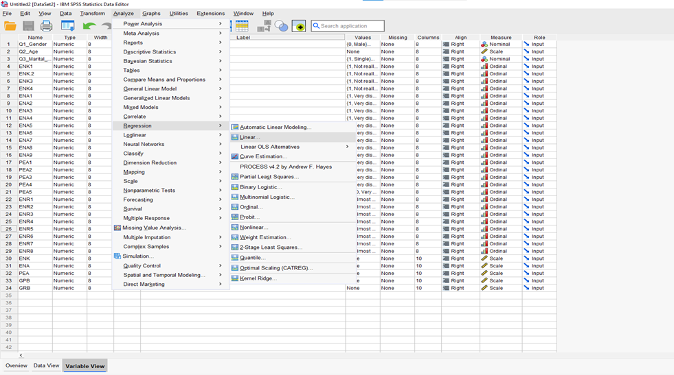
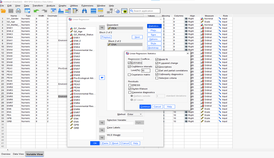
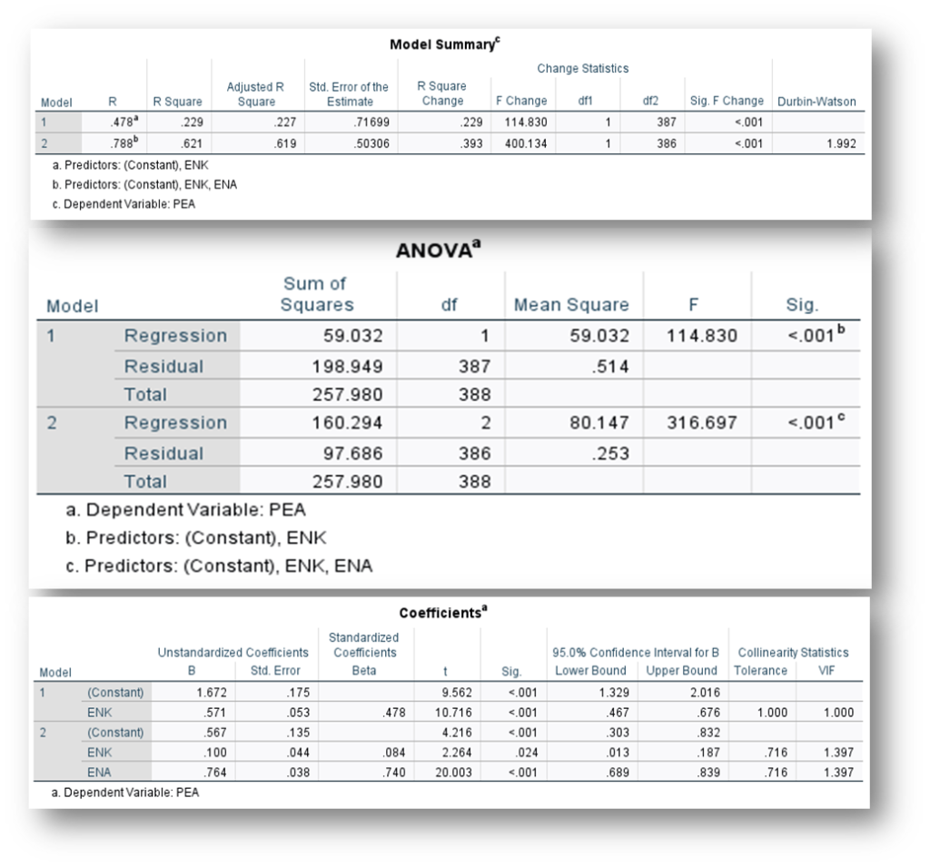
Go to Analyze >> Regression >> Linear (Figure 3.1) >> [move the mean scores of Environmental Knowledge—(ENK) and Environmental Awareness—(ENA) to “Block box = Independent Variable(s) box” (i.e., ENK for Block 1 and ENA for Block 2 by clicking on next)andmean score of “Pro-Environmental Attitude—PEA” must move to “Dependent Variable” box (Figure 3.2) and >> Statistics (check: R-square change, Part and partial correlations, Collinearity diagnostics, Confident Interval (95%), and Durbin-Watson) and rest o of other function just let it defaults, then click Continue (Figure 3.2) >> OK. Then, you will see the following outputs of multiple linear regression for the research hypotheses (H2) and (H3) [i.e., Figure 3.3]. Refer to the outputs (shown in Table 5) of the H2 and H3 below:
This study proposes the research hypotheses, as followed:
Hypothesis (H2): “Environmental Knowledge” has a positive influence on “Pro-Environmental Attitude.”
Hypothesis (H3): “Environmental Awareness” has a positive influence on “Pro-Environmental Attitude.”

Figure 3.1. Multiple Linear Regression [Linear]–[Will update this section soon]

Figure 3.2. Multiple Linear Regression [Options]
2.3. Output of Multiple Linear Regression–[Will update this section soon]

2.4. Table 5. The Result of Hypothesis (H2) and (H3)–[Will update this section soon]
| Independent variables | Dependent variable: Pro-Environmental Attitudes—(Y1) | |
| β1 (Model-1) | β2 (Model-2) | |
| Environmental Knowledge (X1) | 0.084** | |
| Environmental Awareness (X2) | 0.740*** | |
| R2 (R-square) | 0.229 | 0.621 |
| Adjusted-R2 | 0.227 | 0.619 |
| F-value (Significant of p-value) | 114.830 (p<0.001) | 316.697 (p<0.001) |
| t-value | 2.264 | 20.003 |
| p-value | 0.025 <0.05 | <0.001 |
| Durbin-Watson (D-W) | 1.992 | 1.992 |
| VIF | 1.397 | 1.397 |
| Confident Interval (CI) | [0.013 – 0.187] | [0.689 – 0.829] |
| d.f (Regression) | 1 | 2 |
| d.f (Residual) | 387 | 386 |
Note: ***p<0.001, **p<0.05, *p<0.10 and significant at t-value > |1.96|, d.f= degree of freedom
The interpretation of multiple regression is similar to simple regression because simple regression is a special case of multiple regression (Doane & Seward, 2016). Multiple linear regression analysis was conducted to evaluate the extent to which “Environmental Knowledge” and “Environmental Awareness” could predict “Pro-Environmental Attitudes” of local tourism community. In Model-1, a significant regression was found F (1,387) = 114.820, p< 0.001). The R2 was 0.229, indicating “Environment Knowledge” explained approximately 22.9% of the variance in “Pro-Environmental Attitudes”. In Model-2, a significant regression was found F (2,386) = 316.697, p < 0.001). The R2 was 0.621, indicating “Environment Awareness” explained approximately 62.1% of the variance in “Pro-Environmental Attitudes”. Thus, the multiple regression equation in was:
$$Y_1(EPA)=\beta_0+\beta_1X_1(ENK)+\beta_2X_2(ENA)+\varepsilon_0\;\;(Equation\;4)$$
$$Then:Y_1(EPA)=1.672+0.084ENK+0.740ENA+0.175\;\;(Equation\;4)$$
That is, for increase in “Environmental Knowledge”, the predicted “Pro-Environmental Attitudes” increased by approximately 0.013 or 13%. Confidence intervals indicated that we can be 95% certain that the slope to predict “Environmental Knowledge” from “Pro-Environmental Attitudes “is between 0.013 and 0.187. The regression coefficients showed that for “Pro-Environmental Attitudes” increased by an average of 0.084 (8.4%) (β1 = 0.084, SE = 0.175, t = 2.264, p =0.024< 0.05). This result indicated that “Pro-Environmental Attitudes” are a significant predictor of “Environmental Knowledge”, supporting the hypothesis that increased “Environmental Knowledge” is associated with “Pro-Environmental Attitudes”. Overall, the findings suggest that encouraging local tourism community to engage in more “Environmental Knowledge” could enhance their “Pro-Environmental Attitudes”.
Similarly, for increase in “Environmental Awareness”, the predicted “Pro-Environmental Attitudes” increased by approximately 0.689 or 68.9%. Confidence intervals indicated that we can be 95% certain that the slope to predict “Environmental Awareness” from “Pro-Environmental Attitudes “is between 0.689 and 0.928. The regression coefficients showed that for “Pro-Environmental Attitudes” increased by an average of 0.621 (62.1%) (β2 = 0.740, SE = 0.135, t = 20.003, p < 0.001). This result indicated that “Pro-Environmental Attitudes” are a strongly significant predictor of “Environmental Awareness”, supporting the hypothesis that increased “Environmental Awareness” is associated with “Pro-Environmental Attitudes”. Overall, the findings suggest that encouraging local tourism community to engage in more “Environmental Awareness” could enhance their “Pro-Environmental Attitudes”. In summary, the goal of multiple regression analysis is to identify which independent variables have the greatest influence on predicting the dependent variable. Thus, the results indicate that “environmental awareness” is the most significant factor influencing “pro-environmental” attitudes, accounting for 62.1%. This means that if researchers wish to change the behavior or attitudes of the local tourism community, they would gain more knowledge and awareness about the environments.
2.5. Step by Step: Multiple Linear Regression (Updated version: 17-Dec-2024)
2.6. References
1.-Anderson, D. R., Sweeney, D. J., Williams, T. A., Freeman, J., & Shoesmith, E. (2014). Statistics for business and economics (12th ed.). Cengage 2.-Learning, Inc.
3.-Doane, D. P., & Seward, L. W. (2016). Applied statistics in business and economics. Mcgraw-Hill.
4.-Groebner, D. F., Shannon, P. W., & Fry, P. C. (2018). Business statistics: A decision-making approach. Pearson.
5.-Hair Jr, J., Black, W., Babin, B., & Anderson, R. (2019). Multivariate data analysis: A global perspective. Prentice Hall and Pearson.
6.-Hair Jr, J. F., Hult, G. T. M., Ringle, C. M., & Sarstedt, M. (2021). A primer on partial least squares structural equation modeling (PLS-SEM). Sage publications.
7.-Johnston, R., Jones, K., & Manley, D. (2018). Confounding and collinearity in regression analysis: a cautionary tale and an alternative procedure, illustrated by studies of British voting behavior. Quality & Quantity, 52(4), 1957-1976. https://doi.org/10.1007/s11135-017-0584-6
Step 1: Prepare Your Data
1. Open SPSS and load your dataset.
2. Ensure that your dependent variable (the outcome you want to predict) is continuous, and your independent variables (the predictors) can be continuous or categorical.
Step 2: Conduct Multiple Regression Analysis
1. In SPSS, click on Analyze in the top menu.
2. Select Regression, and then choose Linear.
3. In the Linear Regression dialog box:
– Move your dependent variable into the Dependent box.
– Move your independent variables into the Independent(s) box.
4. Click on the Statistics button to select additional outputs, such as:
– Estimates: This will give you information about the coefficients.
– Model fit: This includes R², Adjusted R², and other statistics.
– Descriptive and Durbin-Watson: These statistics can help examine multicollinearity and autocorrelation, respectively.
– Click Continue when you are done selecting options.
5. (Optional) Click on the Plots button if you want to create diagnostic plots, such as scatterplots of residuals versus predicted values to check for homoscedasticity.
6. Click OK to run the analysis.
Step 3: Interpret the Output
SPSS will generate a series of tables in the output window
1. Model Summary Table:
This table contains important information about the regression model such as:
– R: The correlation coefficient indicating the strength of the relationship.
– R²: The coefficient of determination, which indicates the proportion of variance in the dependent variable explained by the independent variables.
– Adjusted R²: Adjusts R² for the number of predictors in the model, providing a more accurate measure of goodness-of-fit.
2. ANOVA Table:
This table tests the overall significance of the regression model. It includes the F-statistic and its significance level (p-value). A significant p-value (typically <0.05) indicates that at least one independent variable significantly predicts the dependent variable.
3. Coefficients Table:
This table provides the unstandardized and standardized coefficients (B and Beta), t-statistics, and p-values for each independent variable.
– The unstandardized coefficient (B) shows the expected change in the dependent variable for a one-unit increase in the independent variable, assuming all other variables are held constant.
– The significance level (p-value) determines whether the independent variable is a significant predictor of the dependent variable. A p-value less than 0.05 typically indicates statistical significance.
4. Example Interpretation
1. If R² = 0.65, this means that 65% of the variance in the dependent variable is explained by the independent variables included in the model.
2. If one of your independent variables has a coefficient (B) of 3.2 and a p-value of 0.01, you would interpret this as: for every one-unit increase in this predictor, the dependent variable is expected to increase by 3.2 units, and this relationship is statistically significant.
3. If a variable has a p-value greater than 0.05, you might consider that variable not statistically significant in the model.

Leave a Reply