Running a simple regression analysis in SPSS allows you to examine the relationship between a dependent variable and one independent variable. By following these steps, you can successfully perform and interpret a simple regression analysis in SPSS, allowing you to determine the relationship between your variables of interest.

I. PURPOSES

Simple and multiple regression analysis in SPSS is used to understand relationships between variables and make predictions based on those relationships (Groebner et al., 2018). Both analyses can be performed using the built-in regression functions, allowing users to easily input data, choose variables, and interpret results through output tables and graphs. Used in various fields such as social sciences, marketing, health research, and any discipline where understanding or predicting relationships among variables is important.

II. SIMPLE LINEAR REGRESSION

In simple linear regression, each observation consists of two variables: one for the independent variable and one for the dependent variable (Anderson et al., 2014).

• To assess the relationship between one independent variable (predictor) and one dependent variable (outcome).
• Key Uses:
• Predicting the value of the dependent variable based on the independent variable.
• Understanding the strength and direction of the relationship (positive or negative).
• Calculating the effect size and assessing the significance of the predictor variable.
• Rules and Guidelines:
• Sample Size: A minimum of 15-20 observations for each predictor variable is often recommended. However, more data is preferable to achieve reliable results.
• Linearity: The relationship between the independent and dependent variable should be linear. This can be visually assessed using scatter plots.
• Normality: Residuals (errors) should be approximately normally distributed, especially for inference tests (like t-tests on regression coefficients).
• Homoscedasticity: The variance of residuals should be constant across all levels of the independent variable(s). This means that the spread of residuals should not increase or decrease as predicted values increase.

III. CONCEPTUAL FRAMEWORK AND HYPOTHESES DEVELOPMENT

Table 1. Summary of Hypotheses Development

Research Constructs	Independent Variables (X)	Mediating Variables (MEV)	Dependent Variables (Y)
Direct Effects
H1: ENK–>ENA	Environmental Knowledge		Environmental Awareness
H2: ENK–>PEA	Environmental Knowledge		Pro-Ecological Attitudes
H3: ENA–>PEA	Environmental Awareness		Pro-Ecological Attitudes
H4: PEA –>ENR	Pro-Ecological Attitudes		Environmental Responsibility
Indirect Effects
H5: ENK–> PEA –> ENR	Environmental Knowledge	Pro-Ecological Attitudes	Environmental Responsibility
H4: ENA –> PEA –> ENR	Environmental Awareness	Pro-Ecological Attitudes	Environmental Responsibility

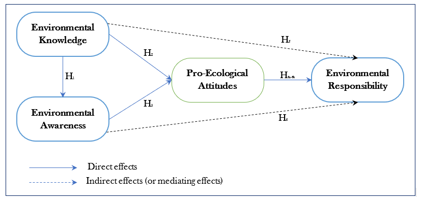
Figure 1. Proposed conceptual framework

1. RULE OF THUMBS: REGRESSION ANALYSIS

Table 2. The Rule of Thumbs: Regression Analysis

Criterion	Threshold Values
R2 (R-square)	≥ 0.10 (10%)
Adjusted- R2	≥ 0.10 (10%)
F-value	≥ 4
t-value	≥ |1.96|
p-value	< 0.05
Durbin-Watson (D-W)	[1.50-2.50]
VIF	≤ 2.5

Sources: Hair Jr et al., 2019; Hair Jr et al., 2021; Johnston et al., 2018

2. EQUATION OF SIMPLE REGRESSION

$$Y_1=\beta_0+\beta_1X_1+\varepsilon_0\:\:\:\:\:(Equation\;1.1)$$

Where:

– β₀ is an intercept or constant value
– β₁ is a slope of regression line or (curve) direction
– X₁: is the value of independent variable
– Y₁: is the value of dependent variable
– ε₀ is is the standardized error or random error term

Example 1:

In the above conceptual framework, our research hypothesis (H₁) is to predict the relationship between “Environmental Knowledge” and “Environmental Awareness”. Therefore, the following equation of simple regression will be:

$$ENA=\beta_0+\beta_1\;ENK+\varepsilon_{0\;}\;\;\;\;(Equation\;1.2)$$

Where:

– β₀ is an intercept or constant value
– β₁ is a slope of regression line or (curve) direction
– X₁: is the value of independent variable (Environmental Knowledge: ENK)
– Y₁: is the value of dependent variable (Environmental Awareness: ENA)
– ε₀ is is the standardized error or random error term

3. STEP BY STEP: SIMPLE LINEAR REGRESSION

PART I. SIMPLE REGRESSION ANALYSIS FOR A SINGLE FACTOR

Go to Analyze >> Regression >> Linear (Figure 1.1) >> [move the mean score of “Environmental Knowledge—ENK” to “Block box = Independent Variable(s) box” and​mean score of “Environmental Awareness—ENA” must move to “Dependent Variable” box  (Figure 1.2) and  >> Statistics (check: R-square change, Part and partial correlations, Collinearity diagnostics, Confident Interval (95%), and Durbin-Watson) and rest o of other function just let it defaults, then click Continue (Figure 1.2) >> OK. Then, you will see the following outputs of simple regression analysis for the research hypothesis (H1).  Refer to the outputs (Figure 1.3) and shown in (Table 3) of the H1 below and more details of this step by step, refer to Appendix:

Hypothesis (H1): Environmental Knowledge has a positive influence on Environmental Awareness.

1.1. Outputs of Simple Linear Regression [Hypothesis 1]–[Will update this section soon]

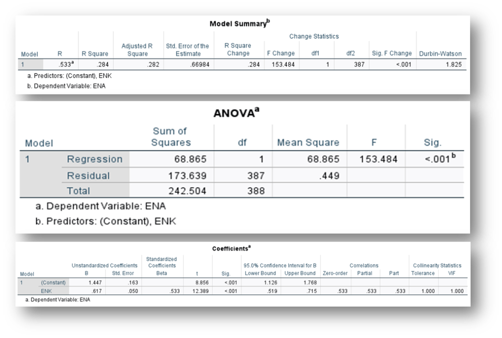
Figure 1.3. The Results of Simple Regression Analysis

1.2. Table 3. The Result of Simple Linear Regression for a Single Factor–[Will update this section soon]

Independent Variable	Dependent Variable
	Environmental Responsibility (Y1)
	β1 (Model-1)
Environmental Knowledge (X1)	0.533***
R2 (R-square)	0.284
Adjusted-R2	0.282
F-value (Significant of p-value)	153.484 (p<0.001)
t-value	12.389
p-value	<0.001
Durbin-Watson (D-W)	1.825
VIF	1.00
Confident Interval (CI)	[0.519 – 0.715]
d.f (Regression)	1
d.f (Residual)	387

Note:

^***p<0.001, ^**p<0.05, ^*p<0.10 and significant at t-value > |1.96|.

d.f= degree of freedom.

R²= Beta Correlation Coefficient (β₁)² (i.e., β₁= (0.533)² = 0.284 (R²)

Simple linear regression analysis was conducted to evaluate the extent to which “Environmental Knowledge” could predict “Environmental Awareness” of local tourism community. A significant regression was found F(1,387) = 153.484, p = < 0.001). The R² was 0.284, indicating “Environmental Knowledge” explained approximately 28.4% of the variance in “Environmental Awareness”.  The simple regression equation in Model-1 was:

$$Y_1(ENK)=\beta_0+\beta_1X_1(ENA)+\varepsilon_0\;\;\;\;(Equation\;1)$$

$$Then:Y_1(ENK)=1.447+0.533PEA+0.163\;\;\;\;(Equation\;1)$$

That is, for increase in “Environmental Knowledge”, the predicted “Environmental Awareness” increased by approximately 0.519 or 51.9%. Confidence intervals indicated that we can be 95% certain that the slope to predict “Environmental Awareness” from “Environmental Knowledge “is between 0.519 and 0.715. The regression coefficients showed that for “Environmental Awareness” increased by an average of 0.533 (53.3%) (β₁ = 0.533, SE = 0.163, t = 12.389, p< 0.001). This result indicated that “Environmental Knowledge” are a significant predictor of “Environmental Awareness”, supporting the hypothesis that increased “Environmental Knowledge” is associated with “Environmental Awareness”. Overall, the findings suggest that encouraging local tourism community to engage in more “Environmental Knowledge” could enhance their “Environmental Awareness”. Environmental knowledge significantly impacts environmental awareness in eco-based tourism in Cambodia, promoting sustainable practices and responsible behavior among tourists and locals. This education enhances the overall experience and encourages meaningful engagement with the natural surroundings, empowering both locals and tourists to become environmental stewards.

PART II. SIMPLE REGRESSION ANALYSIS FOR A MULTIPLE FACTORS–[Will update this section soon]

Go to Analyze >> Regression >> Linear (Figure 2.1) >> [move the mean score of “Pro-Environmental Attitude—PEA” to “Block box = Independent Variable(s) box” and​mean score of Environmental Responsibility—(i.e., GPB and GRB) must move to “Dependent Variable” box  (Figure 2.2) and  >> Statistics (check: R-square change, Part and partial correlations, Collinearity diagnostics, Confident Interval (95%), and Durbin-Watson) and rest o of other function just let it defaults, then click Continue (Figure 2.2) >> OK. Then, you will see the following outputs of simple regression analysis for the research hypothesis (H_4a-4b).  Refer to the outputs (shown in Table 4) of the H4a and H4b below:

Attention: In this case, a variable of “Environmental Responsivity “consists of two sub-dimensions (1)- General Protection Behavior—GPB, and (2)-Particular Regulation Behavior—GRB. We already computed mean score of these factors in SPSS data set.   Therefore, we will have two simple regression results with Hypothesis (H_4a) and (H_4b). Let’s break down the relationship of this hypothesis below. Based on this break down relationships, we need to run the simple regression twice. First, to test the relationship between H_4a and second, to the test the relationship between H_4b.

Hypothesis (H4a): “Pro-Environmental Attitude” has a positive influence on “General Protection Behavior.”
Hypothesis (H4b): “Pro-Environmental Attitude” has a positive influence on “Particular Regulation Behavior.”

Figure 2. Two Factors of Environmental Responsibility

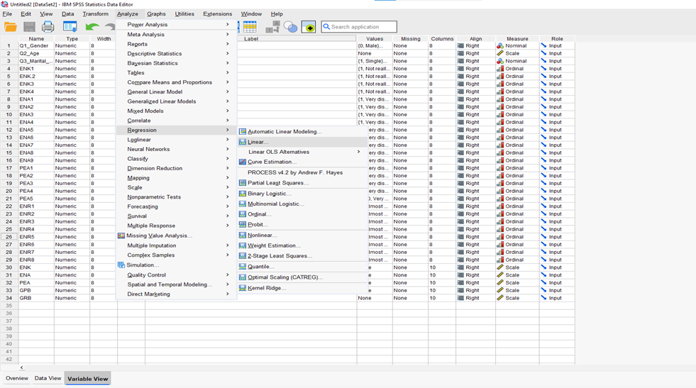
Figure 2.1. Simple regression analysis [Linear]–[Will update this section soon]

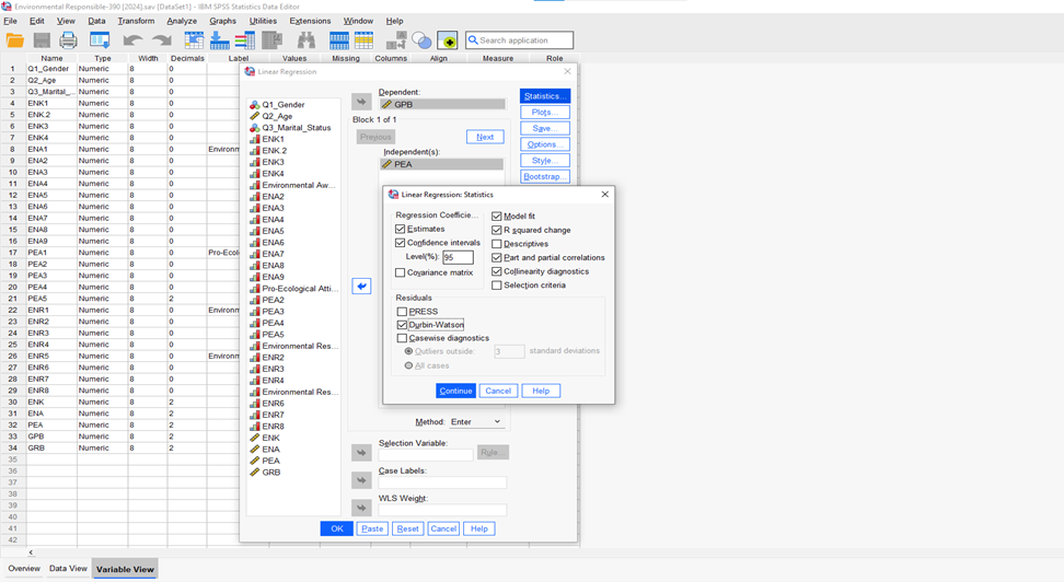
Figure 2.2. Simple regression analysis [Option]

4. Output of Simple Linear Regression for Hypothesis (H_4a)–[Will update this section soon]

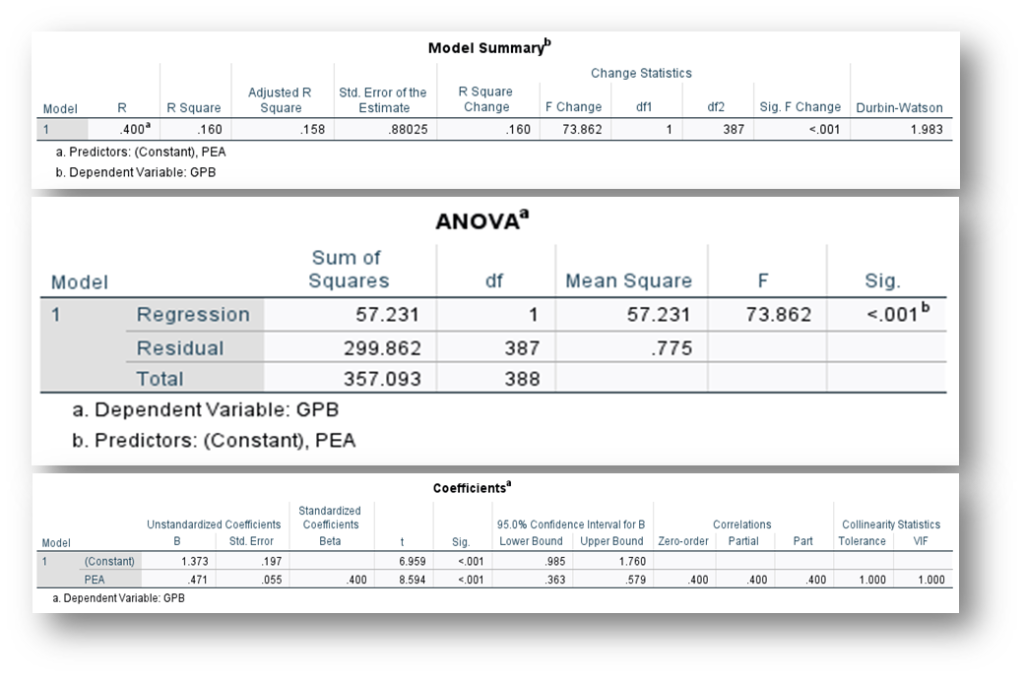
5. Output of Simple Linear Regression: Outputs—For Hypothesis (H_4b)–[Will update this section soon]

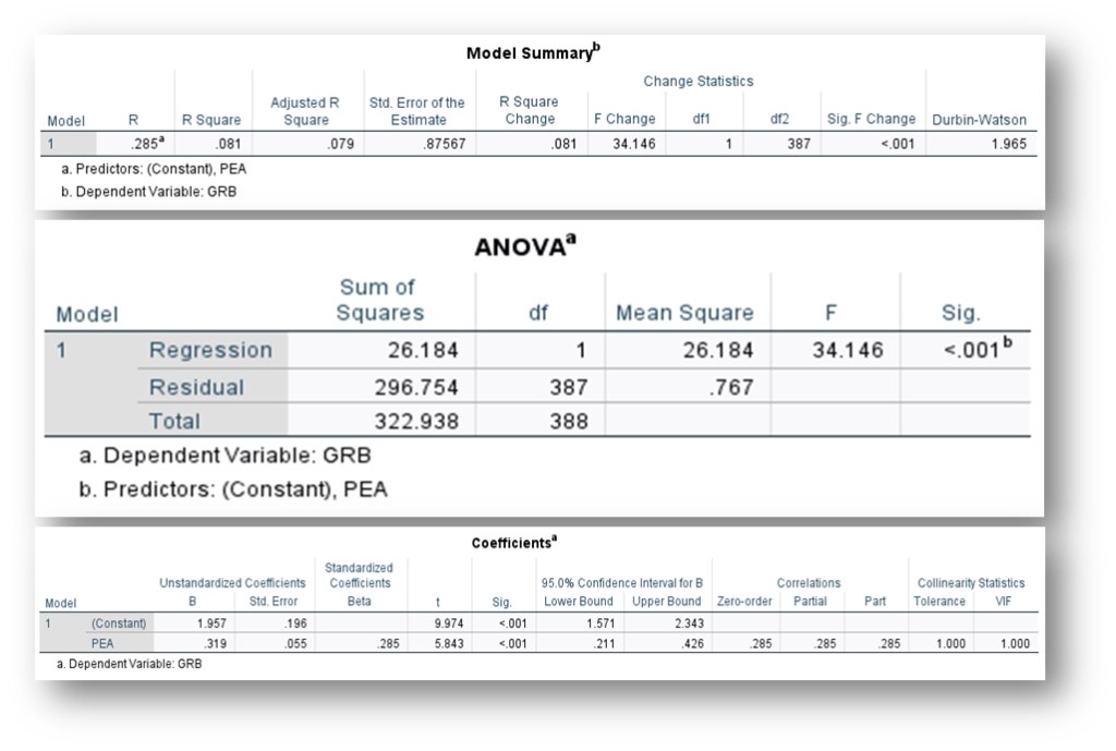
6. Table 4. The Results of Simple Linear Regression for Multiple Factors [(H_4a) and (H_4b)]–[Will update this section soon]

Independent Variable	Dependent Variable:  Environmental Responsibility
	Green Protection Behavior (Y1)	Green Responsible Behavior (Y2)
	β1 (Model-1)	β2 (Model-2)
Pro-Environmental Attitudes (X1)	0.400***	0.285***
R2 (R-square)	0.160	0.081
Adjusted-R2	0.158	0.079
F-value (Significant of p-value)	73.862 (p<0.001)	34.146 (p<0.001)
t-value	8.594	5.843
p-value	<0.001	<0.001
Durbin-Watson (D-W)	1.983	1.965
VIF	1.00	1.00
Confident Interval (CI)	[0.363 – 0.579]	[0.211 – 0.426]
d.f (Regression)	1	1
d.f (Residual)	387	387

Note: ^***p<0.001, ^**p<0.05, ^*p<0.10 and significant at t-value > |1.96|. d.f = Degree of freedom

7. RESULTS AND INTERPRETATION [Will update this section soon]

7.1. For Hypothesis (H_4b)

Simple linear regression analysis was conducted to evaluate the extent to which “Pro-Environmental Attitudes” could predict “Green Protected Behavior” of local tourism community. A significant regression was found F(1,387) = 73.862, p< 0.001). The R² was 0.160, indicating “Pro-Environmental Attitudes” explained approximately 16% of the variance in “Green Protected Behavior”.  The simple regression equation in Model-1 was:

$$Y_1(GPB)=\beta_0+\beta_1X_1(PEA)+\varepsilon_0\;\;\;\;(Equation\;2)$$

$$Then:Y_1(GPB)=1.373+0.400PEA+0.197\;\;\;(Equation\;2)$$

That is, for increase in “Pro-Environmental Attitudes”, the predicted “Green Protected Behavior” increased by approximately 0.363 or 36.3%. Confidence intervals indicated that we can be 95% certain that the slope to predict “Green Protected Behavior” from “Pro-Environmental Attitudes “is between 0.363 and 0.579. The regression coefficients showed that for “Green Protected Behavior” increased by an average of 0.400 (40.0%) (β₁ = 0.400, SE = 0.197, t = 8.594, p < 0.001). This result indicated that “Pro-Environmental Attitudes” are a significant predictor of “Green Responsible Behavior”, supporting the hypothesis that increased “Pro-Environmental Attitudes” is associated with “Green Responsible Behavior”. Overall, the findings suggest that encouraging local tourism community to engage in more “Pro-Environmental Attitudes” could enhance their “Green Protected Behavior”.

7.2. For Hypothesis (H_4a)

Simple linear regression analysis was conducted to evaluate the extent to which “Pro-Environmental Attitudes” could predict “Green Responsible Behavior” of local tourism community. A significant regression was found F (1,387) = 34.146, p < 0.001). The R² was 0.081, indicating “Pro-Environmental Attitudes” explained approximately 8.1% of the variance in “Green Responsible Behavior”.  The simple regression equation in Model-2 was:

$$Y_1(GRB)=\beta_0+\beta_1X_1(PEA)+\varepsilon_0\;\;\;(Equation\;3)$$

$$Then:Y_1(GRB)=1.957+0.258PEA+0.196\;\;\;(Equation\;3)$$

That is, for increase in “Pro-Environmental Attitudes”, the predicted “Green Responsible Behavior” increased by approximately 0.211 or 21.1%. Confidence intervals indicated that we can be 95% certain that the slope to predict “Green Protected Behavior” from “Pro-Environmental Attitudes “is between 0.211 and 0.426. The regression coefficients showed that for “Green Responsible Behavior” increased by an average of 0.258 (25.8%) (β₁ = 0.258, SE = 0.196, t = 5.843, p < 0.001). This result indicated that “Pro-Environmental Attitudes” are a significant predictor of “Green Responsible Behavior”, supporting the hypothesis that increased “Pro-Environmental Attitudes” is associated with “Green Responsible Behavior”. Overall, the findings suggest that encouraging local tourism community to engage in more “Pro-Environmental Attitudes” could enhance their “Green Responsible Behavior”. Therefore, the results show a very weak relationship between “pro-environmental attitudes” and “green responsible behavior,” with an 8.1% correlation. This means that among 390 participants, there are only 32 respondents (i.e., [390×0.081] = 32) who have the concepts of “green responsible behavior” in their local tourism community.

8. APPENDIX: STEP BY STEP FOR REGRESSION ANALYSIS (Update version: 17-Dec-2024)

9. REFERENCES

1.-Anderson, D. R., Sweeney, D. J., Williams, T. A., Freeman, J., & Shoesmith, E. (2014). Statistics for business and economics (12th ed.). Cengage Learning, Inc.
2.-Doane, D. P., & Seward, L. W. (2016). Applied statistics in business and economics. McGraw-Hill.
3.-Groebner, D. F., Shannon, P. W., & Fry, P. C. (2018). Business statistics: A decision-making approach. Pearson.
4.-Hair Jr, J., Black, W., Babin, B., & Anderson, R. (2019). Multivariate data analysis: A global perspective. Prentice Hall and Pearson.
5.-Hair Jr, J. F., Hult, G. T. M., Ringle, C. M., & Sarstedt, M. (2021). A primer on partial least squares structural equation modeling (PLS-SEM). Sage publications.
6.-Johnston, R., Jones, K., & Manley, D. (2018). Confounding and collinearity in regression analysis: a cautionary tale and an alternative procedure, illustrated by studies of British voting behavior. Quality & Quantity, 52(4), 1957-1976. https://doi.org/10.1007/s11135-017-0584-6

11. SUPPLEMENTARY DOCUMENTS

Step 1: Prepare Your Data
1. Open SPSS and load your dataset.
2. Ensure that your dependent variable (the outcome you want to predict) and independent variable (the predictor) are correctly formatted. The dependent variable should be continuous (interval or ratio), while the independent variable can be continuous or categorical.
Step 2: Conduct Simple Regression Analysis
1. In SPSS, go to the menu and click on Analyze.
2. Select Regression, and then choose Linear.
3. In the Linear Regression dialog box:
– Move your dependent variable to the Dependent box.
– Move your independent variable to the Independent(s) box.
4. Click on the Statistics button to select additional statistics:
– Check options such as Estimates, Model fit, R squared change, and Descriptive for additional outputs, if desired.
– Click Continue when done.
5. Optionally, you can click on Plots if you want to create diagnostic plots for residuals. For example, you can create a scatter plot of the residuals to check for homoscedasticity.
6. Click OK to run the regression analysis.
Step 3: Interpret the Output
SPSS will generate several tables in the output window:
1. Model Summary:
– This table provides the R, R² (coefficient of determination), and Adjusted R² values, which indicate the proportion of variance in the dependent variable that can be explained by the independent variable(s).
– R² values range from 0 to 1 (higher values indicate a better fit).
2. ANOVA Table:
– This table tests the overall significance of the regression model. It contains the F-statistic and associated p-value. If the p-value is less than 0.05 (or your chosen alpha level), it indicates that the model significantly predicts the dependent variable.
3. Coefficients Table:
– This table displays the regression coefficients (B values) for the intercept and independent variable(s). It also shows the Standard Error, t-statistic, and p-value for each predictor.
– The coefficient for the independent variable indicates the expected change in the dependent variable for a one-unit change in the independent variable, assuming all other variables are held constant.
– The significance level (p-value) indicates whether the predictor is statistically significant. A p-value less than 0.05 typically indicates statistical significance.
Example Interpretation
1. If your regression output shows an R² value of 0.45, this indicates that 45% of the variance in the dependent variable can be explained by the independent variable.
2. If the coefficient for the independent variable is 2.5 with a p-value of 0.03, this suggests that for each one-unit increase in the independent variable, the dependent variable is expected to increase by 2.5 units, and this relationship is statistically significant.

Step 1: Prepare Your Data
1. Open SPSS and load your dataset.
2. Ensure that your dependent variable (the outcome you want to predict) and independent variable (the predictor) are correctly formatted. The dependent variable should be continuous (interval or ratio), while the independent variable can be continuous or categorical.
Step 2: Conduct Simple Regression Analysis
1. In SPSS, go to the menu and click on Analyze.
2. Select Regression, and then choose Linear.
3. In the Linear Regression dialog box:
– Move your dependent variable to the Dependent box.
– Move your independent variable to the Independent(s) box.
4. Click on the Statistics button to select additional statistics:
– Check options such as Estimates, Model fit, R squared change, and Descriptive for additional outputs, if desired.
– Click Continue when done.
5. Optionally, you can click on Plots if you want to create diagnostic plots for residuals. For example, you can create a scatter plot of the residuals to check for homoscedasticity.
6. Click OK to run the regression analysis.
Step 3: Interpret the Output
SPSS will generate several tables in the output window:
1. Model Summary:
– This table provides the R, R² (coefficient of determination), and Adjusted R² values, which indicate the proportion of variance in the dependent variable that can be explained by the independent variable(s).
– R² values range from 0 to 1 (higher values indicate a better fit).
2. ANOVA Table:
– This table tests the overall significance of the regression model. It contains the F-statistic and associated p-value. If the p-value is less than 0.05 (or your chosen alpha level), it indicates that the model significantly predicts the dependent variable.
3. Coefficients Table:
– This table displays the regression coefficients (B values) for the intercept and independent variable(s). It also shows the Standard Error, t-statistic, and p-value for each predictor.
– The coefficient for the independent variable indicates the expected change in the dependent variable for a one-unit change in the independent variable, assuming all other variables are held constant.
– The significance level (p-value) indicates whether the predictor is statistically significant. A p-value less than 0.05 typically indicates statistical significance.
Example Interpretation
1. If your regression output shows an R² value of 0.45, this indicates that 45% of the variance in the dependent variable can be explained by the independent variable.
2. If the coefficient for the independent variable is 2.5 with a p-value of 0.03, this suggests that for each one-unit increase in the independent variable, the dependent variable is expected to increase by 2.5 units, and this relationship is statistically significant.